
Interventions
Temporarily change disturbance, target, or learning scale.
IRAM-Ω-Q / Inside the simulation
How the simulation works
An agent regulates its internal uncertainty while the world keeps changing. Step inside the loop—and see what its state and regulatory effort reveal.
Explore the simulation
What does it take for an adaptive system to remain organized under uncertainty?
01 / The model
State is only part of the story.
Two agents may reach similar internal states while one needs substantially more corrective control. IRAM-Ω-Q makes that difference visible by tracking both the regulated state and the adaptive gain recruited to maintain it.
The framework models uncertainty regulation under stochastic disturbance. Its central comparison is simple: can regulation act before disturbance enters, or only after?
An everyday analogy
Think of a thermostat for uncertainty. The controller compares the current uncertainty with a target and adjusts its response. The aim is a workable internal state—not the elimination of all uncertainty.
Estimate the current internal uncertainty.
Use adaptive control to attenuate incoming exposure.
The current-cycle disturbance enters with regulation available.
Anticipatory regulation (RF). In the foundational and memory studies, regulation before exposure generally requires lower adaptive gain than reactive recovery.

Both orderings share the underlying model and then undergo coherent evolution; the timing of regulation differs. See the full model on page 5.
Inside each run
Choose the target, disturbance, and experimental schedule.
Introduce scheduled interventions or resets, if the experiment calls for them.
Execute the regulation-first or disturbance-first sequence.
Read entropy, coherence gap, gain, and controller change.
Keep measurements aligned with the same time and conditions.
Reading the model
A vector state represents multiple internal alternatives; its density matrix supports entropy and coherence-gap measurements. This “quantum-like” mathematics is a representational tool.

03 / Reading the results
Original plots from the research papers.
Read the two measurements side by side. A state trajectory can look broadly similar even when the controller works harder to sustain it.
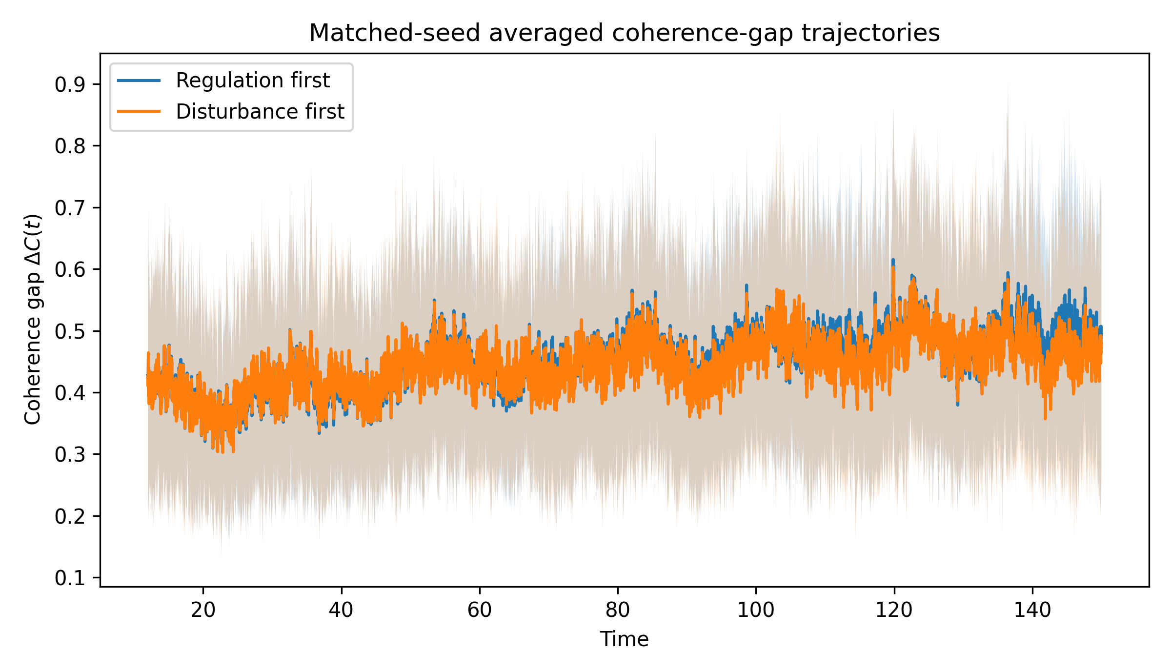
The RF and DF coherence-gap trajectories overlap substantially at the reference setting.
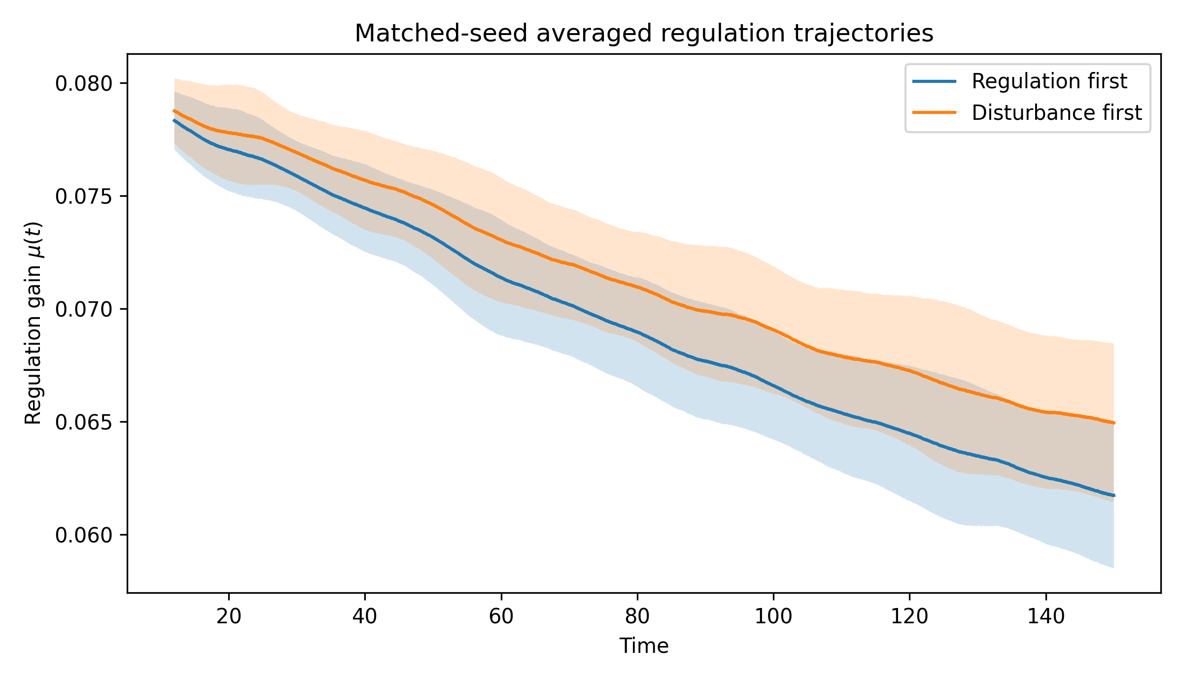
Adaptive gain separates: DF generally recruits more regulation in this comparison.
Finding the sensitive regions
Susceptibility measures temporal variability in the coherence gap after burn-in. Sweeping disturbance and initial gain reveals a ridge where the state becomes especially fluctuation-prone. This is an estimate on the tested grid, not a universal safe threshold.
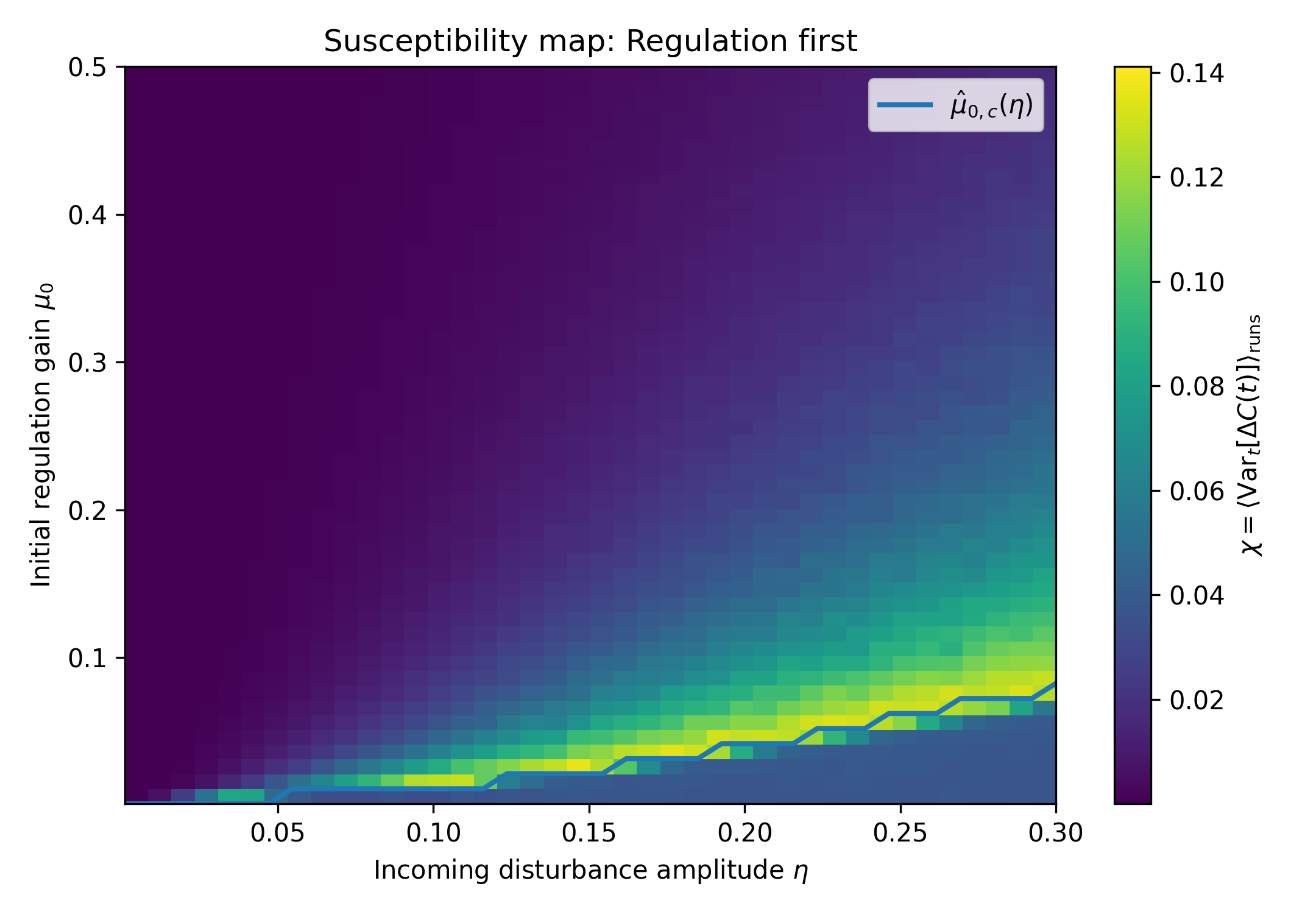
Where coherence-gap fluctuations are greatest under anticipatory regulation.
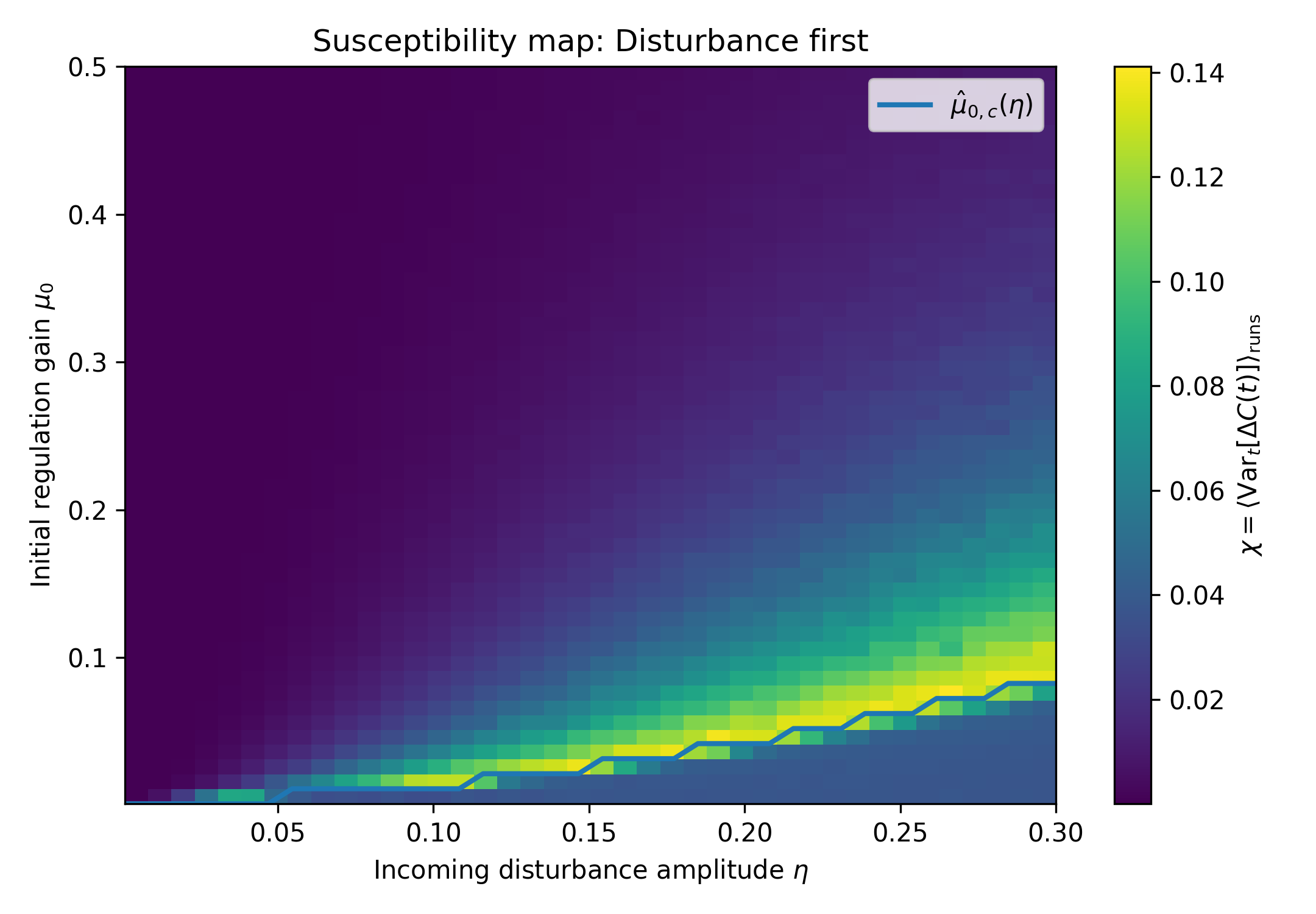
The same measurement under reactive recovery.
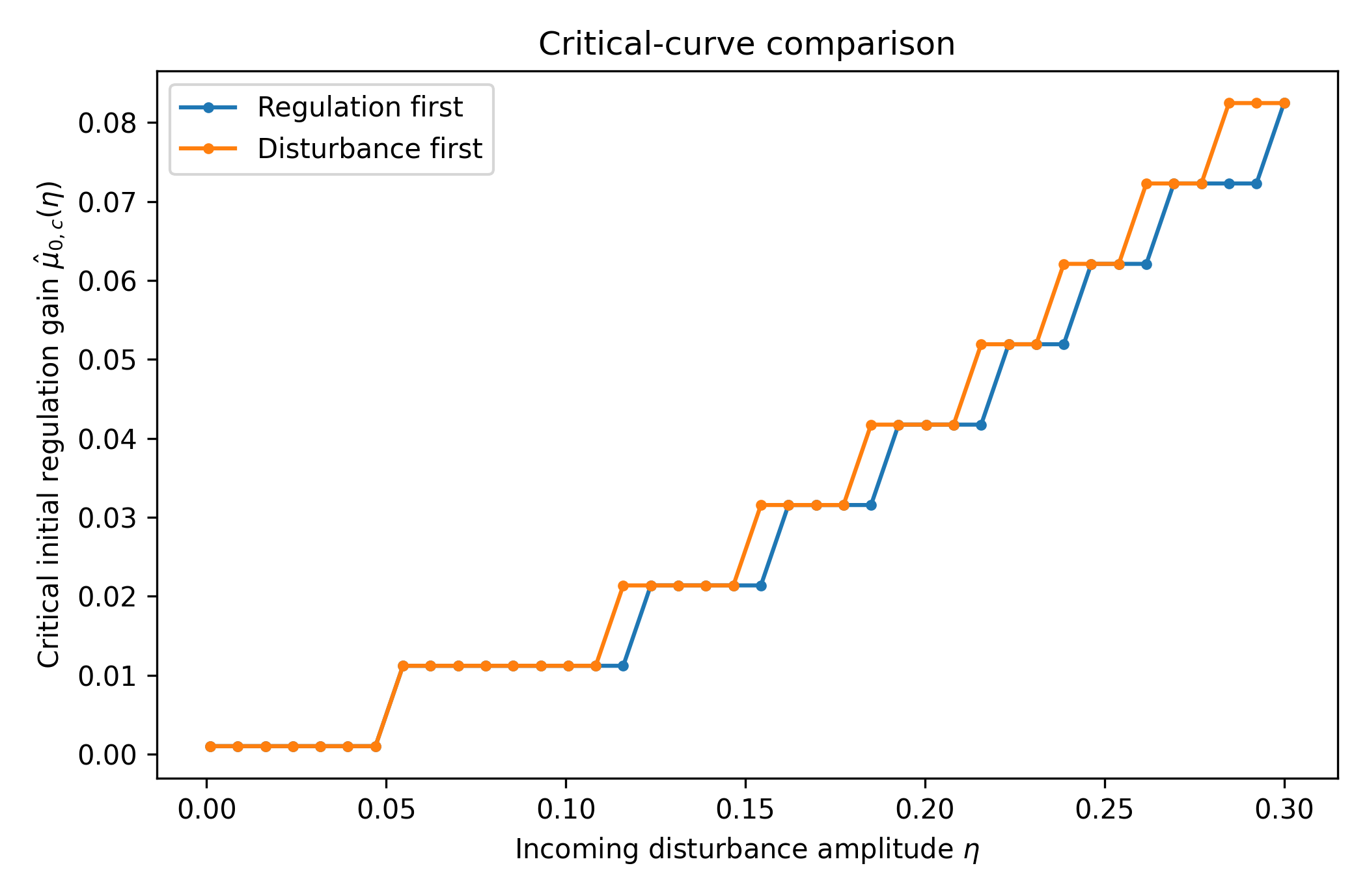
DF shifts parts of the critical ridge toward higher initial gain.
Hysteresis
Move the uncertainty target outward, then reverse it without resetting the agent. Entering and leaving the same target need not trace the same route. This is how the model tests history dependence.
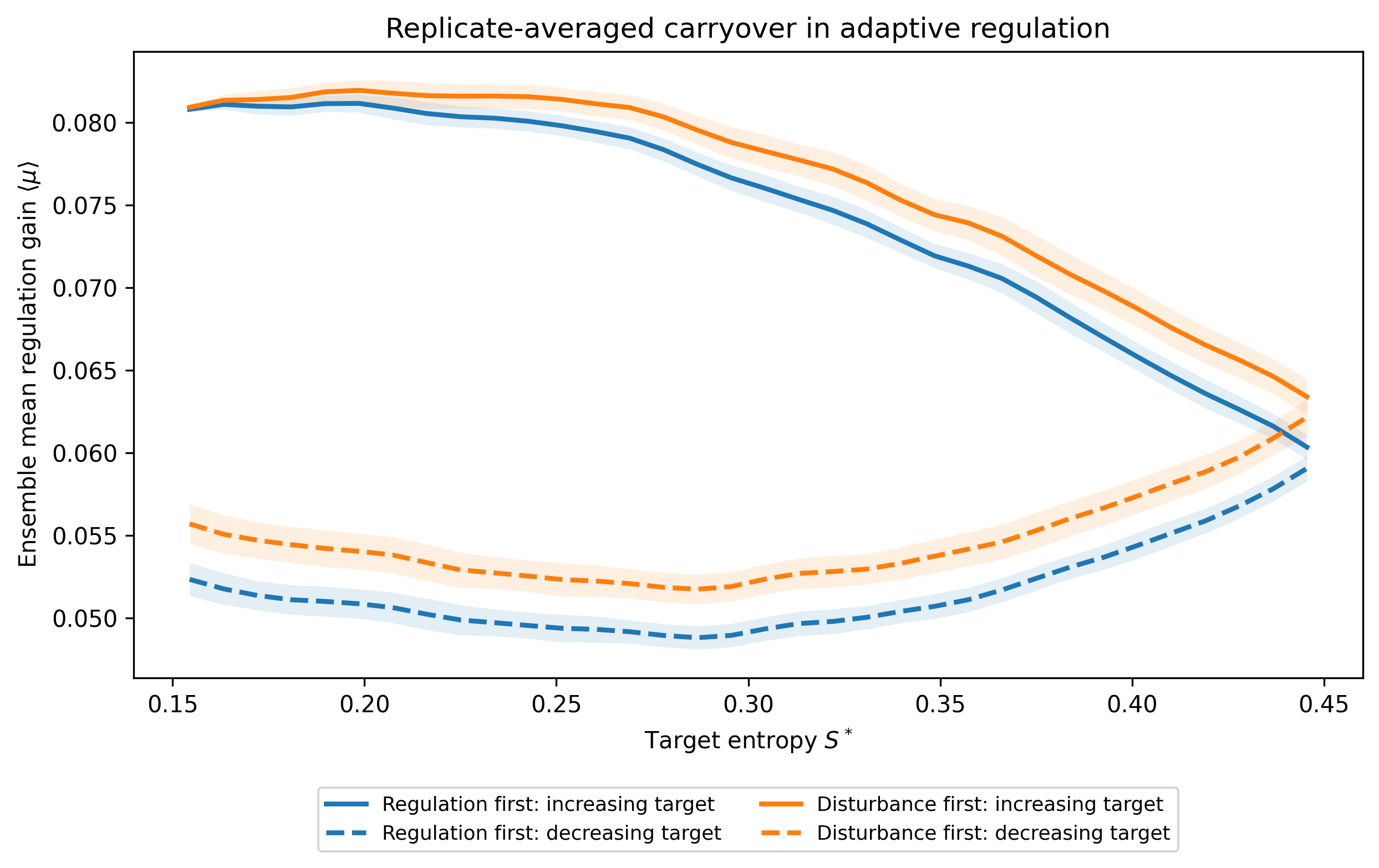
The same target can require different gain depending on the direction of travel.
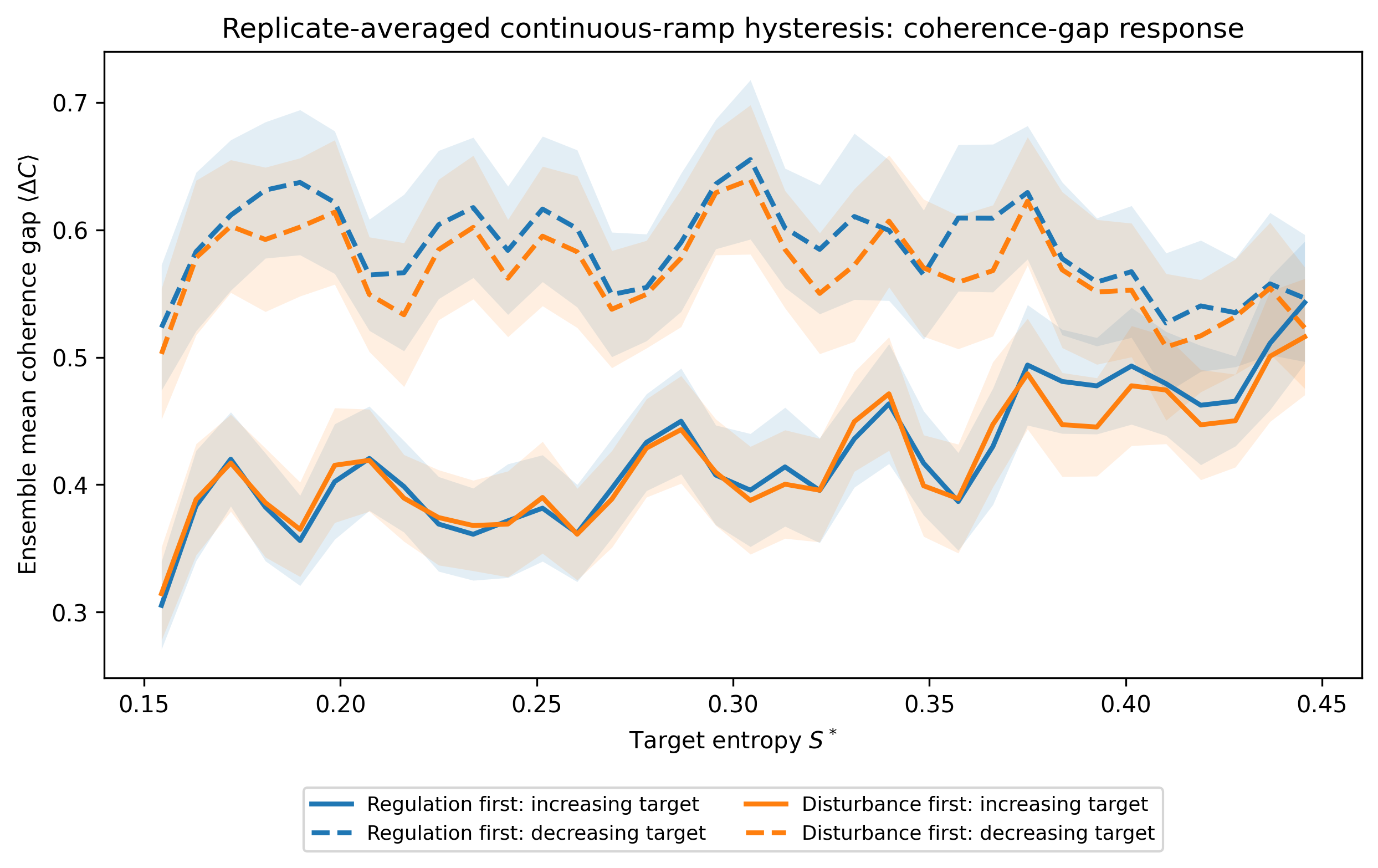
The state also carries history, but the ordering effect is clearer in regulatory gain.
The robustness check
The memory study repeats matched RF/DF comparisons across nine combinations of disturbance and initial gain, with 30 matched pairs at each point.
The clearest consistent ordering effect is in the controller variable μ. Coherence-gap effects are not universal in sign, so the result does not mean one ordering always produces a better state.
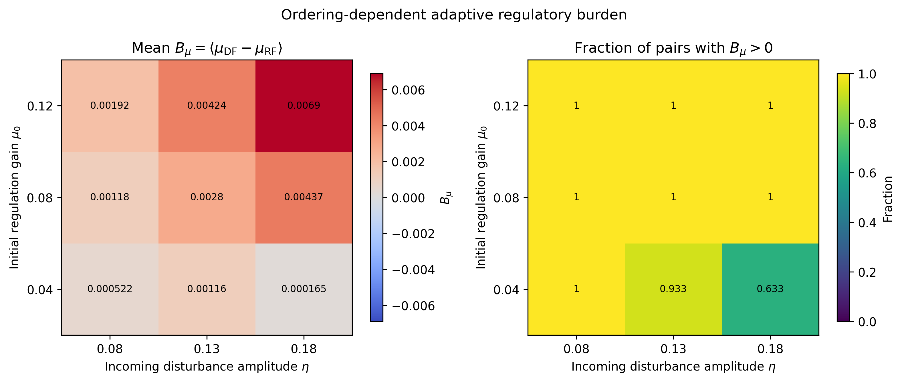
Positive DF-minus-RF gain means that reactive ordering recruited more regulation across the ramp.
04 / When access comes and goes
Intermittent anticipatory regulation
An agent may repeatedly lose and regain anticipatory control. Does that simply average the two fixed modes—or change the later regulatory burden?
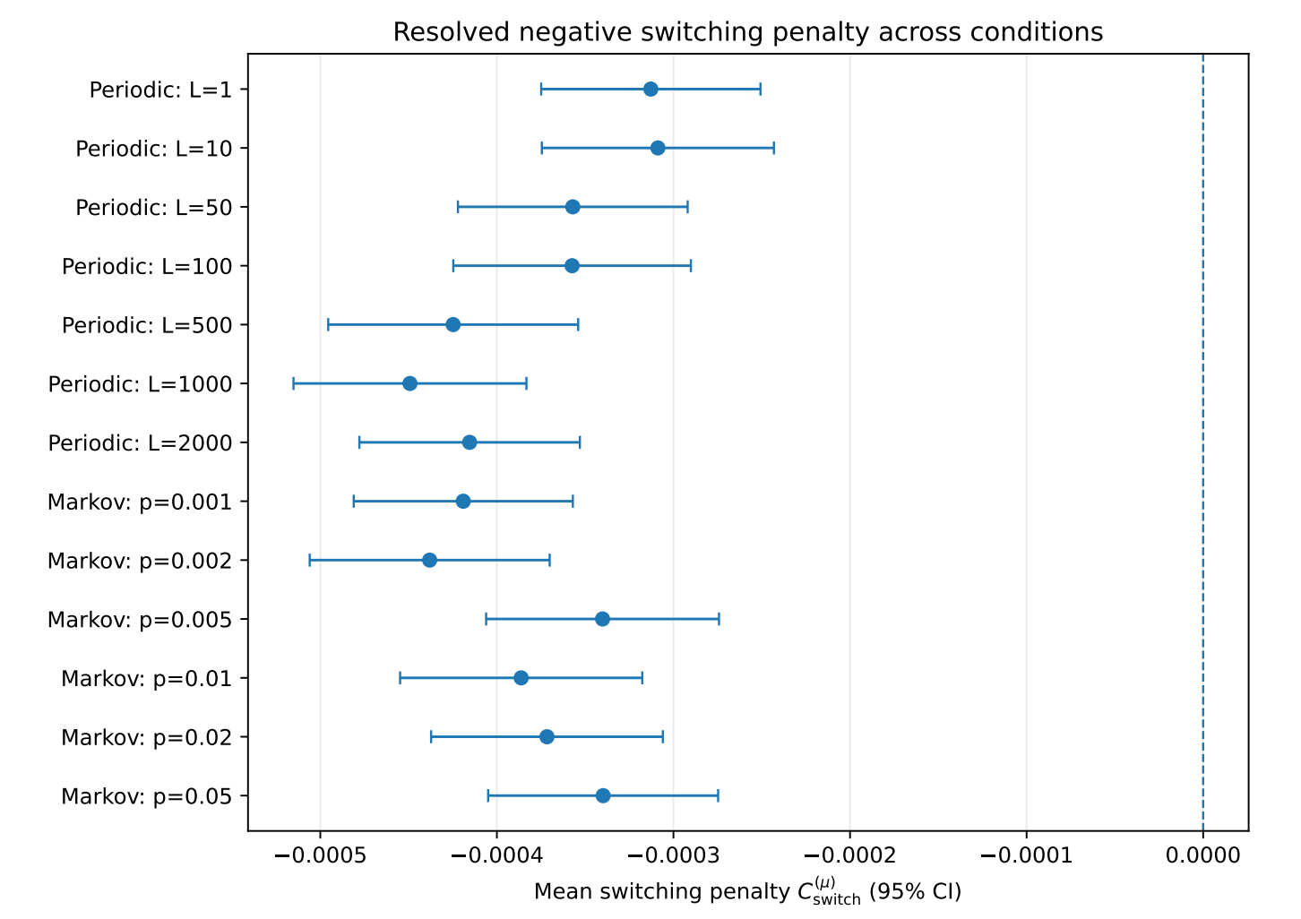
At the reference operating point, every tested periodic and stochastic schedule has a negative mean switching penalty in the high-statistics experiment.
How to read the plot
The baseline combines matched fixed-RF and fixed-DF trajectories according to the time spent in each mode. The switching penalty is the observed mean gain minus that baseline.
At the reference operating point, all tested schedule means lie below zero in the high-statistics result. The effect is small—approximately half a percent of mean gain.
This does not establish that switching outperforms continuous anticipatory control, or that every individual run benefits.
The boundary check
The scan asks whether switching relief persists beyond the reference setting. No tested cell combines a resolved fixed-RF advantage with a resolved positive switching penalty. As the fixed-mode advantage fades, relief can weaken or become statistically unresolved.
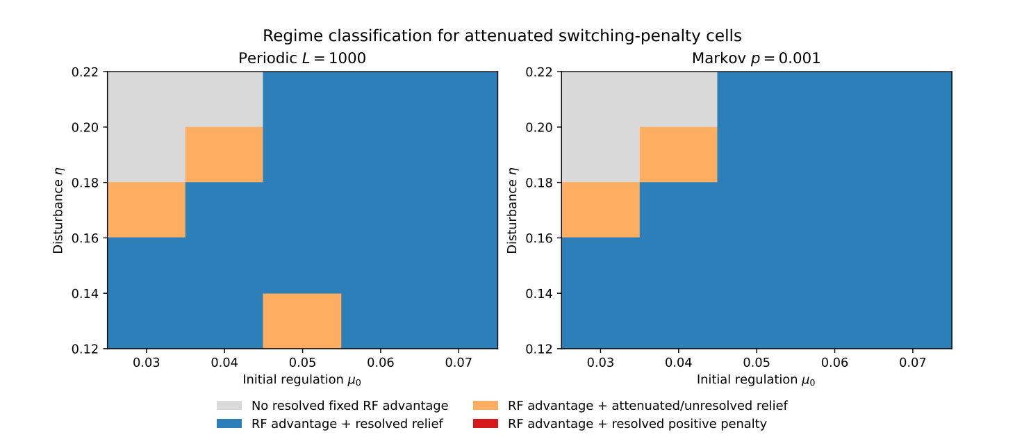
Blue: resolved RF advantage and switching relief. Amber: resolved RF advantage, with attenuated or unresolved switching relief. Gray: no resolved fixed RF advantage.
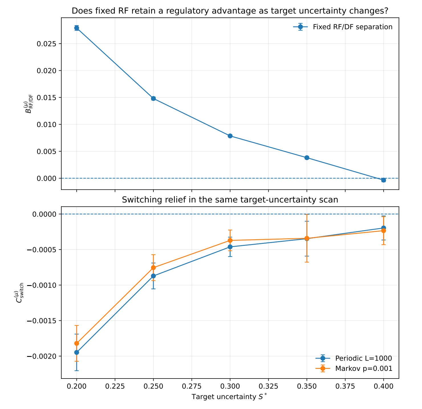
Increasing the target reduces fixed RF/DF separation; switching relief also attenuates toward zero.
05 / A small laboratory
What the workflow makes testable
The same loop supports controlled experiments on regulation, recovery, and the carryover of earlier experience.
Temporarily change disturbance, target, or learning scale.
Reset state, gain, or controller memory to test recovery.
Move the target gradually and reverse it to expose history dependence.
Alternate access to anticipatory regulation while retaining history.
In the induced-cost condition, positive controller updates generate immediate disturbance. The response is nonmonotonic: exposure initially rises, variability increases over an intermediate range, and higher costs can suppress corrective activity.
These findings apply within the tested model and grid; they do not establish a general instability law.
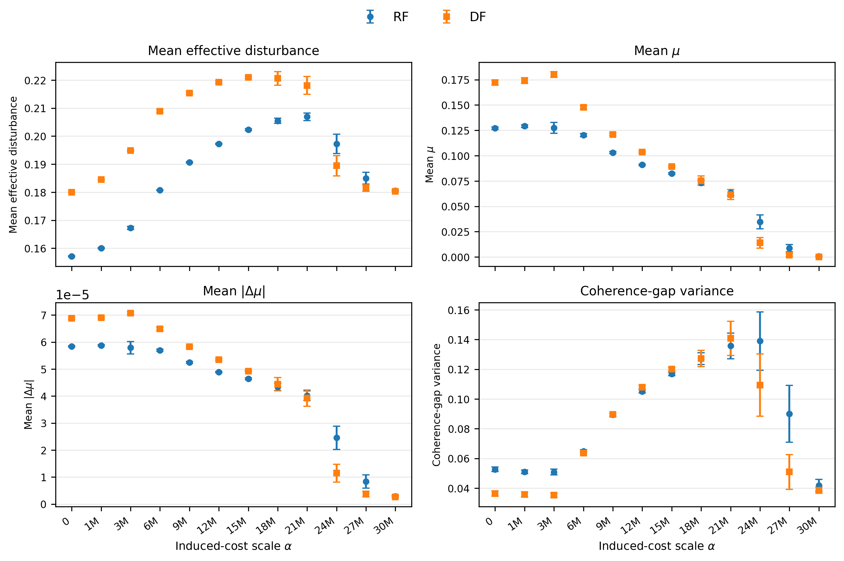
The fourth study extends the workflow to distinguish external, internal, and control-generated disturbance.
06 / The takeaway
IRAM-Ω-Q is a controlled laboratory for adaptive uncertainty regulation.
The agent senses uncertainty, adjusts its regulatory gain, and reveals how its state responds—whether it settles, fluctuates, recovers, or carries history forward.
In the foundational and memory experiments, anticipatory ordering can maintain comparable state-level behavior with lower recruited regulation.
Gain is modeled regulatory demand—not energy, compute cost, or task performance. “Stable” describes the narrative framing, not a formal stability theorem.
The model does not show conscious software, a quantum brain, or universal superiority of regulation-first control.